Analysis Of Algorithm in C++
There are mainly three asymptotic notations:
- Big-O Notation (O-notation)
- Omega Notation (Ω-notation)
- Theta Notation (Θ-notation)
(5):-How to Analyse Loops for Complexity Analysis of Algorithms.
The analysis of loops for the complexity analysis of algorithms involves finding the number of operations performed by a loop as a function of the input size. This is usually done by determining the number of iterations of the loop and the number of operations performed in each iteration.
Here are the general steps to analyze loops for complexity analysis:
Determine the number of iterations of the loop. This is usually done by analyzing the loop control variables and the loop termination condition.
Determine the number of operations performed in each iteration of the loop. This can include both arithmetic operations and data access operations, such as array accesses or memory accesses.
Express the total number of operations performed by the loop as a function of the input size. This may involve using mathematical expressions or finding a closed-form expression for the number of operations performed by the loop.
Determine the order of growth of the expression for the number of operations performed by the loop. This can be done by using techniques such as big O notation or by finding the dominant term and ignoring lower-order terms.
Constant Time Complexity O(1):
The time complexity of a function (or set of statements) is considered as O(1) if it doesn’t contain a loop, recursion, and call to any other non-constant time function.
i.e. set of non-recursive and non-loop statements
In computer science, O(1) refers to constant time complexity, which means that the running time of an algorithm remains constant and does not depend on the size of the input. This means that the execution time of an O(1) algorithm will always take the same amount of time regardless of the input size. An example of an O(1) algorithm is accessing an element in an array using an index.
Example:
- swap() function has O(1) time complexity.
- A loop or recursion that runs a constant number of times is also considered O(1). For example, the following loop is O(1).
Linear Time Complexity O(n):
The Time Complexity of a loop is considered as O(n) if the loop variables are incremented/decremented by a constant amount. For example following functions have O(n) time complexity. Linear time complexity, denoted as O(n), is a measure of the growth of the running time of an algorithm proportional to the size of the input. In an O(n) algorithm, the running time increases linearly with the size of the input. For example, searching for an element in an unsorted array or iterating through an array and performing a constant amount of work for each element would be O(n) operations. In simple words, for an input of size n, the algorithm takes n steps to complete the operation.
Example:
Quadratic Time Complexity O(nc):
The time complexity is defined as an algorithm whose performance is directly proportional to the squared size of the input data, as in nested loops it is equal to the number of times the innermost statement is executed. For example, the following sample loops have O(n2) time complexity
Quadratic time complexity, denoted as O(n^2), refers to an algorithm whose running time increases proportional to the square of the size of the input. In other words, for an input of size n, the algorithm takes n * n steps to complete the operation. An example of an O(n^2) algorithm is a nested loop that iterates over the entire input for each element, performing a constant amount of work for each iteration. This results in a total of n * n iterations, making the running time quadratic in the size of the input.
Example:
(6):-How to analyse Complexity of Recurrence Relation.
The analysis of the complexity of a recurrence relation involves finding the asymptotic upper bound on the running time of a recursive algorithm. This is usually done by finding a closed-form expression for the number of operations performed by the algorithm as a function of the input size, and then determining the order of growth of the expression as the input size becomes large.
Here are the general steps to analyze the complexity of a recurrence relation:
Substitute the input size into the recurrence relation to obtain a sequence of terms.
Identify a pattern in the sequence of terms, if any, and simplify the recurrence relation to obtain a closed-form expression for the number of operations performed by the algorithm.
Determine the order of growth of the closed-form expression by using techniques such as the Master Theorem, or by finding the dominant term and ignoring lower-order terms.
Use the order of growth to determine the asymptotic upper bound on the running time of the algorithm, which can be expressed in terms of big O notation.
It’s important to note that the above steps are just a general outline and that the specific details of how to analyze the complexity of a recurrence relation can vary greatly depending on the specific recurrence relation being analyzed.
In the previous Question, we discussed the analysis of loops . Many algorithms are recursive. When we analyze them, we get a recurrence relation for time complexity. We get running time on an input of size n as a function of n and the running time on inputs of smaller sizes. For example in Merge Sort, to sort a given array, we divide it into two halves and recursively repeat the process for the two halves. Finally, we merge the results. Time complexity of Merge Sort can be written as T(n) = 2T(n/2) + cn. There are many other algorithms like Binary Search, Tower of Hanoi, etc.
need of solving recurrences:
The solution of recurrences is important because it provides information about the running time of a recursive algorithm. By solving a recurrence, we can determine the asymptotic upper bound on the number of operations performed by the algorithm, which is crucial for evaluating the efficiency and scalability of the algorithm.
Here are some of the reasons for solving recurrences:
Algorithm Analysis: Solving a recurrence is an important step in analyzing the time complexity of a recursive algorithm. This information can then be used to determine the best algorithm for a particular problem, or to optimize an existing algorithm.
Performance Comparison: By solving recurrences, it is possible to compare the running times of different algorithms, which can be useful in selecting the best algorithm for a particular use case.
Optimization: By understanding the running time of an algorithm, it is possible to identify bottlenecks and make optimizations to improve the performance of the algorithm.
Research: Solving recurrences is an essential part of research in computer science, as it helps to understand the behavior of algorithms and to develop new algorithms.
Overall, solving recurrences plays a crucial role in the analysis, design, and optimization of algorithms, and is an important topic in computer science.
Introduction to Amortized Analysis
Asymptotic Notations:
(1):- Analysis of Algorithms | Big-O analysis.
Big-O Analysis of Algorithms
We can express algorithmic complexity using the big-O notation. For a problem of size N:
- A constant-time function/method is “order 1” : O(1)
- A linear-time function/method is “order N” : O(N)
- A quadratic-time function/method is “order N squared” : O(N2 )
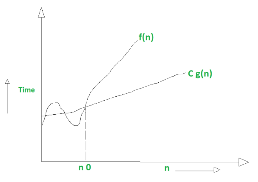
Definition: Let g and f be functions from the set of natural numbers to itself. The function f is said to be O(g) (read big-oh of g), if there is a constant c > 0 and a natural number n0 such that f(n) ≤ cg(n) for all n ≥ n0 .
Note: O(g) is a set!
Abuse of notation: f = O(g) does not mean f ∈ O(g).
The Big-O Asymptotic Notation gives us the Upper Bound Idea, mathematically described below:
f(n) = O(g(n)) if there exists a positive integer n0 and a positive constant c, such that f(n)≤c.g(n) ∀ n≥n0
The general step wise procedure for Big-O runtime analysis is as follows:
- Figure out what the input is and what n represents.
- Express the maximum number of operations, the algorithm performs in terms of n.
- Eliminate all excluding the highest order terms.
- Remove all the constant factors.
Some of the useful properties of Big-O notation analysis are as follow:
Constant Multiplication:
If f(n) = c.g(n), then O(f(n)) = O(g(n)) ; where c is a nonzero constant.
If f(n) = a0 + a1.n + a2.n2 + —- + am.nm, then O(f(n)) = O(nm).
If f(n) = f1(n) + f2(n) + —- + fm(n) and fi(n)≤fi+1(n) ∀ i=1, 2, —-, m,
then O(f(n)) = O(max(f1(n), f2(n), —-, fm(n))).
If f(n) = logan and g(n)=logbn, then O(f(n))=O(g(n))
; all log functions grow in the same manner in terms of Big-O.// C++ program to findtime complexity for single for loop
#include <bits/stdc++.h>
using namespace std;
// main Code
int main()
{
// declare variable
int a = 0, b = 0;
// declare size
int N = 5, M = 5;
// This loop runs for N time
for (int i = 0; i < N; i++) {
a = a + 5;
}
// This loop runs for M time
for (int i = 0; i < M; i++) {
b = b + 10;
}
// print value of a and b
cout << a << ‘ ‘ << b;
return 0;
}
(2):- Difference between Big Oh, Big Omega and Big Theta.
|
S.No. |
Big Oh (O) | Big Omega (Ω) | Big Theta (Θ) |
|---|---|---|---|
| 1. | It is like (<=) rate of growth of an algorithm is less than or equal to a specific value. |
It is like (>=) rate of growth is greater than or equal to a specified value. |
It is like (==) meaning the rate of growth is equal to a specified value. |
| 2. | The upper bound of algorithm is represented by Big O notation. Only the above function is bounded by Big O. Asymptotic upper bound is given by Big O notation. | The algorithm’s lower bound is represented by Omega notation. The asymptotic lower bound is given by Omega notation. | The bounding of function from above and below is represented by theta notation. The exact asymptotic behavior is done by this theta notation. |
| 3. | Big oh (O) – Upper Bound | Big Omega (Ω) – Lower Bound | Big Theta (Θ) – Tight Bound |
| 4. | It is define as upper bound and upper bound on an algorithm is the most amount of time required ( the worst case performance). | It is define as lower bound and lower bound on an algorithm is the least amount of time required ( the most efficient way possible, in other words best case). | It is define as tightest bound and tightest bound is the best of all the worst case times that the algorithm can take. |
| 5. | Mathematically: Big Oh is 0 <= f(n) <= Cg(n) for all n >= n0 | Mathematically: Big Omega is 0 <= Cg(n) <= f(n) for all n >= n0 | Mathematically – Big Theta is 0 <= C2g(n) <= f(n) <= C1g(n) for n >= n0 |
(3):-Examples of Big-O analysis
There are different asymptotic notations in which the time complexities of algorithms are measured. Here, the ”O”(Big O) notation is used to get the time complexities. Time complexity estimates the time to run an algorithm. It’s calculated by counting the elementary operations. It is always a good practice to know the reason for execution time in a way that depends only on the algorithm and its input. This can be achieved by choosing an elementary operation, which the algorithm performs repeatedly, and define the time complexity T(N) as the number of such operations the algorithm performs given an array of length N.
Example 1:
The time complexity for the loop with elementary operations: Assuming these operations take unit time for execution. This unit time can be denoted by O(1). If the loop runs for N times without any comparison. Below is the illustration for the same:
// C++ program to illustrate time
// complexity for single for-loop
#include <bits/stdc++.h>
using namespace std;
// Driver Code
int main()
{
int a = 0, b = 0;
int N = 4, M = 4;
// This loop runs for N time
for (int i = 0; i < N; i++) {
a = a + 10;
}
// This loop runs for M time
for (int i = 0; i < M; i++) {
b = b + 40;
}
cout << a << ‘ ‘ << b;
return 0;
}
Output:
40 160
Explanation: The Time complexity here will be O(N + M). Loop one is a single for-loop that runs N times and calculation inside it takes O(1) time. Similarly, another loop takes M times by combining both the different loops takes by adding them
is O( N + M + 1) = O( N + M).
Example 2:
After getting familiar with the elementary operations and the single loop. Now, to find the time complexity for nested loops, assume that two loops with a different number of iterations. It can be seen that, if the outer loop runs once, the inner will run M times, giving us a series as M + M + M + M + M……….N times, this can be written as N * M. Below is the illustration for the same:
// C++ program to illustrate time
// complexity for nested loop
#include <bits/stdc++.h>
using namespace std;
// Driver Code
int main()
{
int a = 0, b = 0;
int N = 4, M = 5;
// Nested loops
for (int i = 0; i < N; i++) {
for (int j = 0; j < M; j++) {
a = a + j;
// Print the current
// value of a
cout << a << ‘ ‘;
}
cout << endl;
}
return 0;
}
Output:
0 1 3 6 10
10 11 13 16 20
20 21 23 26 30
30 31 33 36 40
Example 3:
After getting the above problems. Let’s have two iterators in which, outer one runs N/2 times, and we know that the time complexity of a loop is considered as O(log N), if the iterator is divided / multiplied by a constant amount K then the time complexity is considered as O(logK N). Below is the illustration of the same:
// C++ program to illustrate time
// complexity of the form O(log2 N)
#include <bits/stdc++.h>
using namespace std;
// Driver Code
int main()
{
int N = 8, k = 0;
// First loop run N/2 times
for (int i = N / 2; i <= N; i++) {
// Inner loop run log N
// times for all i
for (int j = 2; j <= N;
j = j * 2) {
// Print the value k
cout << k << ‘ ‘;
k = k + N / 2;
}
}
return 0;
}
Output:
0 4 8 12 16 20 24 28 32 36 40 44 48 52 56
Example 4:
Now, let’s understand the while loop and try to update the iterator as an expression. Below is the illustration for the same:
// C++ program to illustrate time
// complexity while updating the
// iteration
#include <bits/stdc++.h>
using namespace std;
// Driver Code
int main()
{
int N = 18;
int i = N, a = 0;
// Iterate until i is greater
// than 0
while (i > 0) {
// Print the value of a
cout << a << ‘ ‘;
a = a + i;
// Update i
i = i / 2;
}
return 0;
}
Output:
0 18 27 31 33
Explanation: The equation for above code can be given as:
=> (N/2)K = 1 (for k iterations)
=> N = 2k (taking log on both sides)
=> k = log(N) base 2.
Therefore, the time complexity will be
T(N) = O(log N)
Example 5:
Another way of finding the time complexity is converting them into an expression and use the following to get the required result. Given an expression based on the algorithm, the task is to solve and find the time complexity. This methodology is easier as it uses a basic mathematical calculation to expand a given formula to get a particular solution. Below are the two examples to understand the method.
Steps:
Find the solution for (N – 1)th iteration/step.
Similarly, calculate for the next step.
Once, you get familiar with the pattern, find a solution for the Kth step.
Find the solution for N times, and solve for obtained expression.
Below is the illustration for the same:
Let the expression be:
T(N) = 3*T(N – 1).
T(N) = 3*(3T(N-2))
T(N) = 3*3*(3T(N – 3))
For k times:
T(N) = (3^k – 1)*(3T(N – k))
For N times:
T(N) = 3^N – 1 (3T(N – N))
T(N) = 3^N – 1 *3(T(0))
T(N) = 3^N * 1
T(N) = 3^N
The third and the simplest method is to use the Master’s Theorem or calculating time complexities.
(4):-Difference between big O notations and tilde?
The differences between Big Oh and Tilde notations are :
|
S No- |
Big Oh (O) |
Tilde (~) |
|
1 |
It generally defines the upper bound of an algorithm. |
Since it is similar to theta notation, it defines both the upper bound and lower bound of an algorithm. |
|
2 |
The arbitrary constant incase of Big Oh notation is c which is greater than zero. 0 <= f(n) <= c*g(n) ; c>0, n>=n0
|
Here, the constant will always be 1 since on dividing f by g or g by f we always get 1. So, it gives a sharper approximation of an algorithm.
|
|
3 |
If the time complexity of any algorithm is n^3/3-n^2+1 ,it is given by O(n^3 ) and the constant is ignored.
|
Here, for the same time complexity it will be ~(n^3/3 ). This constant 1/3 is meaningless as in asymptotic analysis we are only interested to know about the growth of a function for a larger value of n.
|
|
4 |
It is mostly used in asymptotic analysis as we are always interested to know the upper bound of any algorithm |
Big theta is mostly used instead of Tilde notation as in case of Big Theta we can have different arbitrary constants, c1 for upper bound and c2 for the lower bound. |
|
5 |
It defines the worst case. |
It mostly defines the average case. |
(5):-Analysis of Algorithms | Big – Ω (Big- Omega) Notation?
Big Omega notation (Ω) :
It is define as lower bound and lower bound on an algorithm is the least amount of time required ( the most efficient way possible, in other words best case).
Just like O notation provide an asymptotic upper bound, Ω notation provides asymptotic lower bound.
Let f(n) define running time of an algorithm;
f(n) is said to be Ω(g (n)) if there exists positive constant C and (n0) such that
0 <= Cg(n) <= f(n) for all n >= n0
n = used to given lower bound on a function
If a function is Ω(n-square) it is automatically Ω(n) as well.
Graphical example for Big Omega (Ω):
(6):- Analysis of Algorithms | Big – Θ (Big Theta) Notation ?
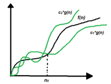
Let g and f be the function from the set of natural numbers to itself. The function f is said to be Θ(g), if there are constants c1, c2 > 0 and a natural number n0 such that c1* g(n) ≤ f(n) ≤ c2 * g(n) for all n ≥ n0
Mathematical Representation:
Θ (g(n)) = {f(n): there exist positive constants c1, c2 and n0 such that 0 ≤ c1 * g(n) ≤ f(n) ≤ c2 * g(n) for all n ≥ n0}
Note: Θ(g) is a set
The above definition means, if f(n) is theta of g(n), then the value f(n) is always between c1 * g(n) and c2 * g(n) for large values of n (n ≥ n0). The definition of theta also requires that f(n) must be non-negative for values of n greater than n0.
Graphical Representation:
In simple language, Big – Theta(Θ) notation specifies asymptotic bounds (both upper and lower) for a function f(n) and provides the average time complexity of an algorithm.
Follow the steps below to find the average time complexity of any program:
- Break the program into smaller segments.
- Find all types and number of inputs and calculate the number of operations they take to be executed. Make sure that the input cases are equally distributed.
- Find the sum of all the calculated values and divide the sum by the total number of inputs let say the function of n obtained is g(n) after removing all the constants, then in Θ notation its represented as Θ(g(n)).